Demand Planning DSS: Forecasting and Regression

Objective Hierarchy

Suppose you want to forecast the demand for your firm’s particular product. What are some variables that might influence it? This is the type of question one asks in trying to model the business situation. Demand drives your entire supply chain – from inventory to distribution to manufacturing and so on. As a business, you want to be able to forecast your demand for the coming period in order to meet your customer needs. All of these will eventually involve interactions with the suppliers and customers. A careful demand planning will not only allow the company to maximize profits and position the company for growth, but it will also help plan short-term and long-term by maintaining durable relationships with their partners. Forecasting demand for your product is necessary to enable your firm to plan its operations (marketing, finance, and manufacturing).

The purpose of this exercise is to become familiar with simple forecasting tool based on statistical analysis of demand history and causal factors such as pricing, advertising and so on. Better demand planning helps you increase forecast accuracy and production efficiency so you can lower your inventory and dramatically improves customer service. The model in this exercise is simple enough to illustrate some of the causes that explain the level of one firm’s demand. It involves the use of time series analysis (here we use CB Predictor), which is a forecasting method that uses historical data to extrapolate some future values in order to create the basis for decision-making. In addition to that, Regression analysis is used to estimate the relationships between variables so that a given variable can be predicted from one or more other variables. These analyses enable us to forecast the next 4 periods for the following variables: Average Demand, Average Price, Average Advertising and Average R&D Expenditure. Then we can create an equation that ultimately predicts the Normalized Share of Market Demand, the dependent variable.

Let us say that the primary objective of the firm is to maximize profit. The following is a graphical representation of the business model that leads to profitability:

Follow this link to find out what each of the node shapes above mean: Influence Diagrams

Variables and Attributes

Demand is expressed as:

Firm Demand = Average Firm Demand (AFD) x Normalized Share of Market (NSOM)

The following two tables describe the variables used to model the demand for the firm.

Influence Diagram

This influence diagram below is a graphical representation of the endogenous and exogenous factors that influence the average firm demand of a particular product.

Mathematical Representation

Average Firm Demand (AFD)

To model this, we need to understand that AFN is influenced by two factors: one is exogenous and the other one is endogenous. This means that the AFD is a function of the trend of the average industry demand and residual that is affected by some independent variables such as average industry prices, average industry advertising, etc. The equation follows that AFN = fitted Trend (Seasonality factored in) + Residual.

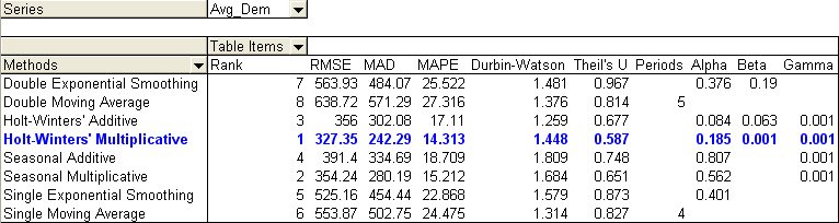
First of all, we need to run a trend analysis on each of the following series: Avg_Dem, Avg_Price, Avg_Adv, Avg_Adv1, Avg_Adv2, Avg_RD1 and Avg_RD2. The last 4 series (Avg_Adv, Avg_Adv1, Avg_Adv2, Avg_RD1 and Avg_RD2) are called lagged variables. A lagged variable is simply the value of an independent variable during the previous period. A two period lag means look at the value of the variable two periods back. To perform time series analysis, CB Predictor is used to select the best method for each of the seven series. Then, CB predictor forecasts the next 10 periods for each of those series. The figure below shows that the Holt-Winters’ Multiplicative Method is the best to perform the trend for Average Demand (Series 1) because of the lowest errors (RMSE, MAD, and MAPE). To see the various models assigned to the series, click here to get the spreadsheet.

RMSE (Root mean squared error): This is an absolute error measure that squares the deviations to keep the positive and negative deviations from canceling each other out. This measure also tends to exaggerate large errors, which can help when comparing methods.

MAD (Mean absolute deviation): This is an error statistic that average distance between each pair of actual and fitted data points.

MAPE (Mean absolute percentage error): This is a relative error measure that uses absolute values to keep the positive and negative errors from canceling each other out and uses relative errors to let you compare forecast accuracy between time-series models

Here’s the chart that shows the trend:

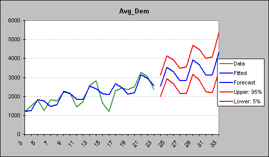
Holt-Winters’ Multiplicative Method accounts for seasonality of 4 quarters. As can be seen from the graph above, the difference between the actual (green) and fitted (blue) data is the residual.

Next, we use the residual data (from period 3 to 23) as a dependent variable and regress it against the independent variables (Avg_Price, Avg_Adv, Avg_RD) to see which of these variables were significant in the prediction. To perform this, we can use Regression tool from Excel Data Analysis. This involves several steps. The first step is to include the three series as the Input X Range (independent variables). Then we look at the P-values of each of those independent variables to determine which one has the highest value. The highest P-value means it is the most insignificant in predicting the dependent variable. The highest P-value in this case is 0.112623885. This variable needs to be removed from the calculation. Before that, I have set the P-value of <= .10 as a useful predictor of the dependent variable.

We run the regression again, but this time, with the Avg_Price and Avg_Adv as the independent variables. This final regression confirms that those two independent variables are significant in the prediction. The R-square value is 0.865175165, meaning that approximately 87% of the variation in Residual is explained by variation in both Average Advertising and Average R&D Expenditure.

The equation for the residual = 18278.20932 -49.71714941 (Avg_Price) + 0.003595112 (Avg_Adv).

Normalized Share of Market (NSOM)

In order to predict the NSOM, we run the regression on the nsom spreadsheet data. We found that all variables are significant. Here’s the result:

The mathematical equation for the Residual Model:

NSOM = 15.94723159 -16.79336984 (Prel) + 0.7312239 (Arel) + 0.444773948 (NSOM1) + 0.178938881 (Rrel1) + 0.256960344 (Rrel2) + 0.152087781 (Arel1) + 0.079412054 (Arel2)

Using all the models from the time series forecasting (trend), AFD residuals and NSOM, a DSS interface model can be developed.

DSS Interface:

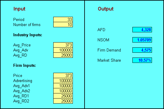
Testing & Validation

This model is designed to calculate the output values for the next 10 periods (period 24 to 33). If the period of higher than 33 is used as input, an error message will appear and no value will result in the output section. The Firm Inputs section tells you about the variables that your firm can control. You will be able to see the effect of over pricing or under pricing on your firm demand. For example, you will lose your market share if you overcharged the price of your product. For the period 24 to 33, the Industry Input values are the forecasted values. Click here to find out the calculations used to produce the output results (click on Calc tab in the spreadsheet)

Implementation & Use

Good Demand Planning provides the corporate management with an effective tool to better manage and optimize the financial and operational performance of their inventory investment. The model we have just seen above could be used as a model within a larger model that interacts with every aspects of business decision making. One good example is that, by changing the inputs in the demand module, it will not only produce the output for the demand, but also the effect on the firm’s financial statements. Essentially, management has to be able to use a powerful system that can meet the objective of the organization, for example, to increase profits by simultaneously maximizing customer service levels, minimizing total annual costs, reducing workloads and reducing inventories. We know that one of the most important aspects of Demand Planning is that all of the departments within a company that use some kind of demand forecast can operate essentially using the same data as every other department. Given that the departments within a corporation can easily work together to obtain a reasonable operating plan, financing and investment plans can also be developed to meet the overall objective of the organization. After all, profit will be determined by the sales revenues and the expenses engaged for R&D and plant construction and so on that involves financing and investment planning.