Prepared by: Vinchel Budihardjo
& Truong D.Vu
Use of
The
usefulness of financial statement projections for corporate financial
management is undisputed. Such projections, called pro forma financial statements, are the bread and butter of much
corporate financial analysis. Pro forma financial statements look at the links
between the balance sheets and income statements and more importantly the flow
of funds in the future. A pro forma income statement is similar to a historical
income statement, except it projects the future rather than tracks the past. It
the projection predicts a downturn in profitability, you can make operational
changes such as increasing prices or decreasing costs before these projections
become reality. A company’s future profitability, borrowing and many other
quantities are all highly uncertain quantities. It seems natural to run a
simulation to obtain a range of values on future profitability and borrowing.
Simulation is related to both scenario and sensitivity analysis. It ties
together sensitivities and input variable probability distributions. We can
play the usual “what-if” games of simulation models, and we can ask what
strains on the firm may be caused by changes in certain variables such as sales
and expenses. The purpose of this exercise is to illustrate the use of Monte Carlo Simulation to form the
basis for valuation and credit analysis. First of all, we need to get the
historical financial statements data for Home Depot and then we create a
simulation.
Relevant Data
Figure 1
below shows the relevant data for Home Depot in 1995. All numbers are in
millions of dollars. Note that Sources = Uses and Assets = Liabilities +
Equities. Given the actual financial statements for Home Depot, we can forecast
their financial statement for the next year (1996). Next year revenue (t+1) is
simply the value of t (current year) multiplied by a constant value shown in
column D. This is the trick in linking year t with the next year (t+1). To see
the key relationships, click here to get the
spreadsheet. Since, the spreadsheet is an @Risk spreadsheet, you also need to
get .rsk file. After running the simulation, both Excel (XLS) and @Risk (RSK)
files need to be saved separately. If the associated .rsk file is not saved,
then reopening an Excel file necessitates rerunning the simulation to obtain
the results.
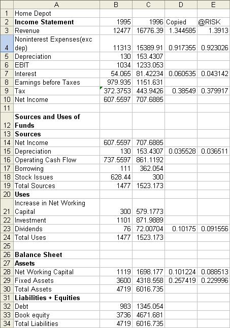
Figure 1
The Dynamics of the Model
In a simulation analysis, the computer begins by
picking at random a value for each of the uncertain variables (Revenue Growth, percentage of Non-interest expenses to
Revenue, Interest rate on Long-Term debt, Tax rate, Depreciation on
Fixed-Assets, Dividend payout rate, Net WC and Fixed Assets) based on
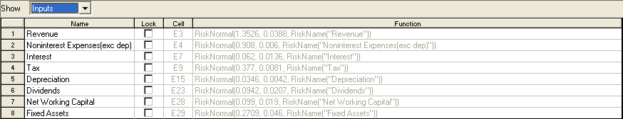
its specified probability distribution. We assign the following names to these
variables: a1-a8.
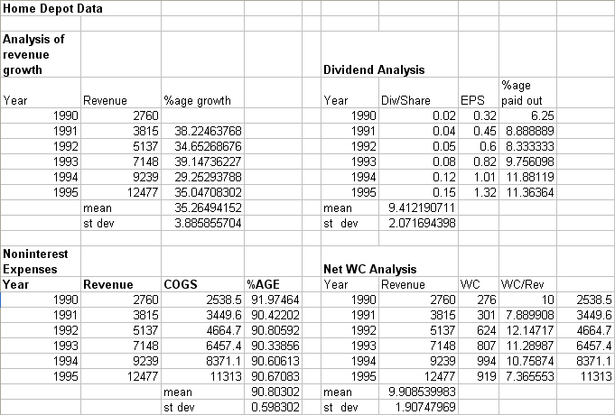
Figure 2
The mean or average value is used as a measure of
expected value and the standard deviation (or coefficient of variation) is used
as a measure of risk. The assumption here is that each of the eight items can
be represented by a continuous random distribution. We make them =RISKNormal functions to model the fact
that each constant may differ in different years. This drives the randomness of
the model. As an example consider a1 (Revenue Growth). This
parameter measure the year to year growth in revenue. For 1991-1995, we found
the average growth in revenue to be 35.26% and the standard deviation to be
3.89%. To model the simulation, we use the formula RiskNormal (1.3526, 0.0388).
The formula for a2 = RiskNormal (0.0991, 0.0191).
Here’s the list of inputs with the formulas assigned:
If you look at the Financial Statement data, you
will notice that net income influences borrowing, borrowing influences debt,
debt influences interest, and interest influences income. In Excel, this is
referred to as circular reference. There is a way of resolving the circular
reference problem. Simply go to “Tools”, then choose “Options” “Calculation”
“Automatic” and check “Iterations” and put in 1000 for maximum iterations. You
will see that Assets = Liabilities + Equities and Uses = Sources.
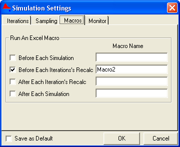
Before running the simulation, we will create a
macro that will paste the constant value (as numbers, not formulas) from the
simulation (column E) to column D. Then it will feed into column C and it will
resolve the circularities. The macro name used is Macro2. Under @Risk
simulation setting, we ask @Risk to run Macro2 before each iteration of a
simulation. The sequence of events would be:
- Run
Macro2
- Compute
@Risk functions and calculate output cells
- Run
Macro2, etc
This ensures that before each time the value of an
output cell is tabulated, new values of a1-a8 will be
generated.
We’re now ready to run the simulation. The only
output we are trying to measure is the Net
Income. After 1000 iterations, @Risk produces the following results:
|
Summary Statistics |
|||
|
Statistic |
Value |
%tile |
Value |
|
Minimum |
505.4887695 |
5% |
674.0304565 |
|
Maximum |
1102.032837 |
10% |
705.9438477 |
|
Mean |
811.5698513 |
15% |
725.0234375 |
|
Std Dev |
85.46608282 |
20% |
743.0560913 |
|
Variance |
7304.451313 |
25% |
755.5171509 |
|
Skewness |
0.039828427 |
30% |
766.8305664 |
|
Kurtosis |
3.216118724 |
35% |
779.039856 |
|
Median |
810.1477051 |
40% |
790.0019531 |
|
Mode |
818.5773621 |
45% |
801.8696289 |
|
Left X |
674.0304565 |
50% |
810.1477051 |
|
Left P |
5% |
55% |
819.0309448 |
|
Right X |
952.2886963 |
60% |
828.7329102 |
|
Right P |
95% |
65% |
840.2873535 |
|
Diff X |
278.2582397 |
70% |
848.4483643 |
|
Diff P |
90% |
75% |
865.7454224 |
|
#Errors |
0 |
80% |
882.7453613 |
|
Filter Min |
|
85% |
900.5479736 |
|
Filter Max |
|
90% |
923.5115967 |
|
#Filtered |
0 |
95% |
952.2886963 |
A picture is worth a thousand words and the summary
statistics above shows the probability distribution of the outcome. We see that
on average, we expect Home Depot’s 1996 Net Income to be 811 million. They
actually made 733 million (according to the actual data), which was in between
the 15th and 20th percentile of what we expected.
@Risk is such a powerful tool in that it gives you
countless reporting and graphing options. To see the complete results, click here.
Conclusion
We can use this simulation technique to forecast as many years ahead as we like. This does not mean it goes with the expectation that past revenue growth assumptions hold. A company could have its business cycle and as such is on S-shaped curve of growth that most companies follow. Also, the industry is expected to become more competitive. This could affect some of the variables we used such as margin (as factored into a2). This model gives you flexibility to build in (with If statements) future assumptions about the industry and the firm behavior (for example: stock issuing policy). In the example above, the revenue growth follows a random normal variable. We could have instead used the other function that takes some of the values as equally likely scenarios of future growth. Let’s say, the revenue growth could be one of the following values: 1.3822, 1.2565, 1.3952, or 1.2585. Instead of using the =RISKNormal function, we could input the function: RISKDUniform({1.3822,1.2565,1.3952,1.2585}) as the formula.
![]()