Situation Description and Objective
This
exercise is based on Example 4.2 (Worker and Production Planning at SureStep)
in the textbook. Most companies need to determine a production schedule in
order to meet the demand of their customers. We will use Excel Solver to plan a production schedule that will minimize total
costs given certain constraints. During the next 4 months, SureStep Company
wants to meet on time the following demands for pairs of shoes:
|
Month |
Pairs
of shoes |
|
1 |
3000 |
|
2 |
5000 |
|
3 |
2000 |
|
4 |
1000 |
Note that
this is the certainty assumption that the company faces. Normally, we do not
know how much to produce in each month given the limited amount of resources
needed to produce the shoes. But, here, for the sake of simplicity, we set the
target to those 4 months values. The following are the input variables to begin
with:
- At the beginning of month 1,
the company has 500 pairs of shoes and 100 workers on hand.
- A worker is paid $1500 per
month
- Each worker can work up to
160 hours per month before he/she receives overtime
- Overtime for each worker is
limited to 20 hours per month and the rate paid per hour of overtime is
$13
- It takes 4 hours of labor and
$15 of raw materials to produce a pair of shoes
- At the beginning of each
month, workers can be hired or fired
- Each hired worker costs
$1600, and each fired worker costs $2000
- If there’s any shoe left in
inventory at the end of the month, holding cost of $3 per pair is incurred
- If the company fails to meet
a unit of demand, a penalty cost of $15 is incurred during each month for
which a shortage occurs

Figure
1
The
solution requires that we keep track of each month’s beginning inventory,
ending inventory, production and all costs
The goal of this spreadsheet is to
determine the optimal production schedule and labor policy
We will
look at some of the variables that
will determine the final output.
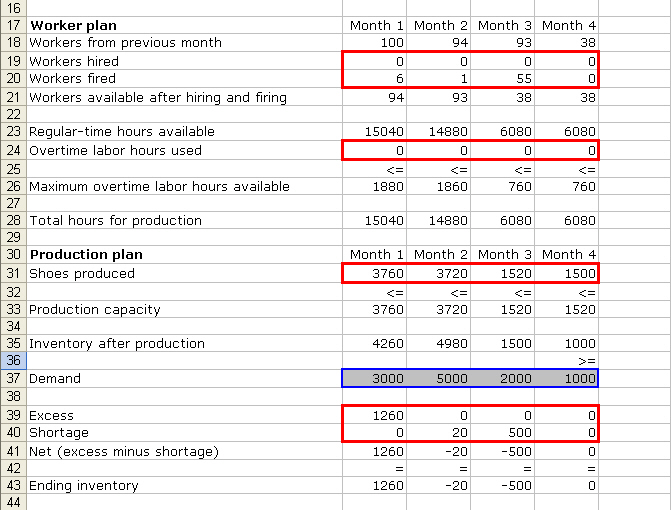
We know
that the company has 100 workers at the beginning of month 1. If they decided
to hire 0 worker and fire 6, then the number of workers available after firing
and hiring = 94. The # of worker to hire and the # of
workers to fire at the beginning of each month are the decision variables. Each
worker has 160 hours per month. Hence, the “regular total hours available” = 94
x 160 = 15040 hours. This does not include the number of overtime labor hours
the company decides to use. Now, we have 96 workers available to produce shoes.
Each worker has overtime limit of 20 hours. The maximum overtime hours
available = 96 x 20 = 1920. Does it mean that the company will use the maximum
overtime hours available? The overtime labor hours
used is the decision variable and it varies from month to month.
Remember that the company wants to use the combination of variables that best
maximize the total profit. Let’s say, the company uses 0 overtime hours. Total
hours used for production = regular total hours available + overtime labor
hours used (15040 = 15040 + 0)
Next, we
determine the “production capacity” by dividing the “number of hours used for
production” by the “number of hours used to produce a pair of shoes.” For
example, if there is 15040 total hours for production and it takes 4 labor
hours to produce a pair of shoes, then the production capacity = 15040/4 = 3760
We know
that the production capacity in month 1 = 3760. Suppose the company decides to
produce 3760 shoes (The decision to produce x number of shoes is the decision
variable). Then “inventory after production” is simply the addition of
last month’s ending inventory (500) to this month’s # of shoes produced (3760).
The demand for the first month is 3000. Ending Inventory is calculated by
subtracting “demand” by “Inventory after production.” If the result is
negative, then it means the company fails to meet the desired demand. A
shortage cost = $15 per unit. If “demand” is less than “inventory after
production,” the company has some shoes left in the inventory that is not sold.
The holding cost = $3 per pair of shoes. This example shows us that the company
has 1260 ending inventory. The cost of holding excess inventory = 1260 x $3 =
$3780.
The
company wants to make sure that by the end of month 4, demand is met. This
means that Ending Inventory in month 4 cannot be negative (the company will not
incur shortage cost). If there’s excess inventory, the company will incur
holding cost. If the ending inventory = 0, the company does not incur any cost.
This is consistent with the idea of minimizing cost.
Figure
2
Click
here to get the spreadsheet
Variables & Attributes
|
Variables |
How Measured |
Related to |
|
# of
workers available after hiring and firing |
Integer |
# of
workers from previous month & hiring of new workers and firing of
existing workers |
|
Regular-time
hours available |
Hours |
# of
workers after hiring and firing & each worker’s hours per month before
receiving overtime |
|
Maximum
overtime labor hours available |
Hours |
# of
workers after hiring and firing & each worker’s 20 overtime hours per
month |
|
Total
hours for production |
Hours |
Regular-time
hours available & Overtime labor hours used |
|
Production
capacity |
Number
of pairs of shoes (cannot be fraction) |
Total
hours for production & # of labor hours required to produce a pair of
shoes |
|
Inventory
after production |
Number
of pairs of shoes (cannot be fraction) |
Prior
month’s ending inventory & # of shoes produced in the current month |
|
Ending
inventory |
Number
of pairs of shoes (cannot be fraction) |
Inventory
after production & # of units demanded |
|
Decision Variables |
How Measured |
Subject to constraints: |
|
# of
workers hired |
Integer |
Value
has to be integer (can not be fraction) |
|
# of
workers fired |
Integer |
Value
has to be integer (can not be fraction) |
|
Overtime
labor hours used |
Hours |
Maximum overtime labor hours available |
|
Shoes
produced |
Number
of pairs of shoes (cannot be fraction) |
Production
capacity |
|
Excess
shoes |
Number
of pairs of shoes (cannot be fraction) |
|
|
Shortage
shoes |
Number
of pairs of shoes (cannot be fraction) |
|
Mathematical Model Formulation
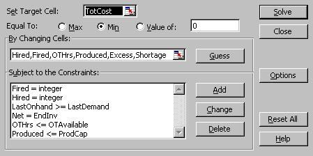
The objective of this linear model is to minimize total costs. Therefore, “total costs” has to
be set as a target cell. We choose
to minimize total costs by adjusting the number of workers hired (B19:E19), the
number of workers fired (B20:E20), the overtime labor hours used (B24:E24) and
the number of shoes to produce (B31:E31). These are the decision variables. The values in these changing cells can be
changed to optimize the objective.
Figure
3
Constraints must be set as follows:
The
number of workers hired & fired must be set as integer (cannot be fraction).
The inventory after production in month 4 must be bigger or equal to the number
of shoes demanded in that month. Overtime labor hours used in each month cannot
exceed the maximum overtime labor hours available. The number of shoes produced
in each month cannot exceed the full production capacity. Net excess minus
shortage equals Ending Inventory. If there’s excess of 10 pairs of shoes, then
there’s no shortage. If there’s excess of -10 pairs of shoes, then shortage =
10 pairs.
The values
in the changing cells cannot be negative.
Development of Spreadsheet Model
We have
already shown the steps to develop the spreadsheet model. The first step is to
enter the values given in the exercise in the input cells (shown in Figure 1). Next,
we input trial values in the changing cells. The formulas for other variables
must also be set. For example, Production capacity in month 1 (B33) = Total
hours for production (B28) x number of labor hours used to produce a pair of
shoes (B12).
Then we
invoke Excel Solver and set it up as shown in Figure 3 (subject to
Constraints). Since this model is a linear model, we go to Options menu and
check both “Assume Linear Model” and “Assume Non-Negative.”
We’re now
ready to tell Solver to find the optimum solution. Clicking Solve button will
do all the jobs in no time.
The final
step is to run sensitivity analysis and see the impact of the increase/decrease
in input variable on the output.
Results
We found
that in order to minimize total costs, we will have to fire some workers in
month 1-3 and hire none in each of the 4 months. Overtime labor hours will not
be used. The company will have to use full production capacity. Finally, we see
that the company will have to incur holding cost in month 1 and shortage cost in
month 2 & 3. There is no shortage or holding cost in the last month because
the company has to meet the demand. The minimum total costs solver found is
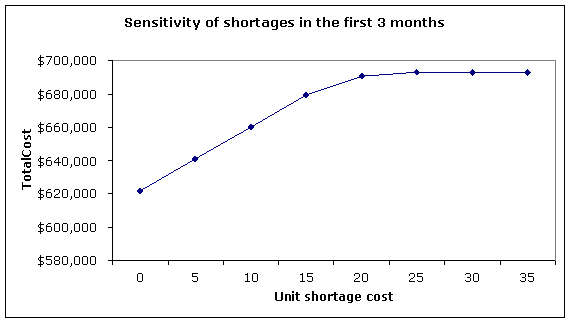
$690,180. Let’s do what-if analysis. Is there any way to decrease the total
costs by changing any of the input variable? We will change the unit shortage
cost (increment of $5) to determine if there is a better alternative for
SureStep.
Sensitivity of
shortages in the first three months and total cost to unit shortage cost
|
Unit
shortage cost |
Shortage1 |
Shortage2 |
Shortage3 |
TotalCost |
|
|
$B$40 |
$C$40 |
$D$40 |
$F$53 |
|
$0 |
0 |
2,280
|
1,640
|
$621,740
|
|
$5 |
0 |
2,220
|
1,580
|
$640,920
|
|
$10 |
0 |
2,220
|
1,580
|
$659,920
|
|
$15 |
0 |
2,220
|
1,580
|
$678,920
|
|
$20 |
0 |
20 |
500 |
$690,180
|
|
$25 |
0 |
20 |
20 |
$692,780
|
|
$30 |
0 |
0 |
0 |
$692,820
|
|
$35 |
0 |
0 |
0 |
$692,820
|
As we
see, when the unit shortage cost is below $20, SureStep is willing to incur
large shortages – at significantly lower total cost. However, shortages become
much less attractive when the unit shortage cost increases, and no shortages
are incurred at all when this unit cost is above $25.
DSS Guidelines & Limitation
This model proves to be simple but useful in assisting labor and production planning. It is essentially every manufacturing company’s problem. The model could be enhanced by including other variables which may prove to be relevant in addressing company’s issues. All in all, this spreadsheet model is a linear model that helps solve the optimal value of an output given certain constraints and formulas that follow it. We have proven that we can use Excel Solver to solve an interesting optimization problem such as this one. We know that the target cell in this model is a linear function of the changing cells. The left-hand and right-hand sides of each constraint are linear functions of the changing cells. When we use the functions =IF, =ABS, =MAX, =MIN which depends on any of the models changing cells, then the model becomes nonlinear. This in turn become an optimization problem for which Excel Solver is ill suited to find optimal solutions. Fortunately, genetic algorithm technique, as discussed in the textbook, can be used as a superior tool to find the optimal solution. The problem becomes more challenging if there’s uncertainty factor in it, such as a demand which is normally distributed with certain monthly mean and standard deviation.